과제링크:Assignment 2 (cs231n.github.io)
Assignment 2
This assignment is due on Monday, May 02 2022 at 11:59pm PST. Starter code containing Colab notebooks can be downloaded here. Setup Please familiarize yourself with the recommended workflow before starting the assignment. You should also watch the Colab wa
cs231n.github.io
내 풀이 링크: https://github.com/lionkingchuchu/cs231n.git
GitHub - lionkingchuchu/cs231n: cs231n Spring 2022 Assignment
cs231n Spring 2022 Assignment. Contribute to lionkingchuchu/cs231n development by creating an account on GitHub.
github.com
Assignment 2의 첫번째 Q1 과제는 FullyConnectedNets로 Assignment 1의 마지막 과제였던 TwoLayerNet을 이제는 Two Layer가 아닌 여러개의 Layer을 가진 FCNets를 만들어 보는 과제이다. Assignment Q2, Q3: batch normalization, dropout 이 같은 파일을 사용해서 batch norm, dropout 내용이 포함되어 있다.
class FullyConnectedNet(object):
    """Class for a multi-layer fully connected neural network.

    Network contains an arbitrary number of hidden layers, ReLU nonlinearities,
    and a softmax loss function. This will also implement dropout and batch/layer
    normalization as options. For a network with L layers, the architecture will be

    {affine - [batch/layer norm] - relu - [dropout]} x (L - 1) - affine - softmax

    where batch/layer normalization and dropout are optional and the {...} block is
    repeated L - 1 times.

    Learnable parameters are stored in the self.params dictionary and will be learned
    using the Solver class.
    """

    def __init__(
        self,
        hidden_dims,
        input_dim=3 * 32 * 32,
        num_classes=10,
        dropout_keep_ratio=1,
        normalization=None,
        reg=0.0,
        weight_scale=1e-2,
        dtype=np.float32,
        seed=None,
    ):

        self.normalization = normalization
        self.use_dropout = dropout_keep_ratio != 1
        self.reg = reg
        self.num_layers = 1 + len(hidden_dims)
        self.dtype = dtype
        self.params = {}


        # *****START OF YOUR CODE (DO NOT DELETE/MODIFY THIS LINE)*****

        for x in range(1,self.num_layers+1):
          if x == 1:
            self.params['W'+str(x)] = np.random.randn(input_dim, hidden_dims[x-1]) * weight_scale
            self.params['b'+str(x)] = np.zeros([hidden_dims[x-1],])
            if normalization == 'batchnorm':
              self.params['gamma'+str(x)] = np.ones_like(self.params['b'+str(x)])
              self.params['beta'+str(x)] = np.zeros_like(self.params['b'+str(x)])
            continue

          if x == self.num_layers:
            self.params['W'+str(x)] = np.random.randn(hidden_dims[x-2], num_classes) * weight_scale
            self.params['b'+str(x)] = np.zeros([num_classes,])
            continue

          self.params['W'+str(x)] = np.random.randn(hidden_dims[x-2], hidden_dims[x-1]) * weight_scale
          self.params['b'+str(x)] = np.zeros([hidden_dims[x-1],])
          if normalization == 'batchnorm':
            self.params['gamma'+str(x)] = np.ones_like(self.params['b'+str(x)])
            self.params['beta'+str(x)] = np.zeros_like(self.params['b'+str(x)])

        # *****END OF YOUR CODE (DO NOT DELETE/MODIFY THIS LINE)*****
위의 설명처럼 FullyConnectedNets는 [affine - (batch/layer norm) - relu - (dropout)] 형태의 layer가 L-1개, 그리고 마지막의 affine layer까지 합해 총 L개의 layer을 가지고 있는 network이다. 먼저 self.num_layer의 개수 만큼 affine layer을 위한 parameter들 W1, b1, W2... 를 만들어 준다. 만약 batch normalization 또는 layer normalization을 사용한다면, (normalization == 'batchnorm') normalization의 parameter: gamma 와 beta를 마지막 affine layer을 제외한 layer 개수만큼 만들어준다. dropout layer은 parameter를 사용하지 않으므로 dropout을 사용한다 하더라도 별도의 parameter를 만들 필요가 없다.
    def loss(self, X, y=None):

        X = X.astype(self.dtype)
        mode = "test" if y is None else "train"

        # Set train/test mode for batchnorm params and dropout param since they
        # behave differently during training and testing.
        if self.use_dropout:
            self.dropout_param["mode"] = mode
        if self.normalization == "batchnorm":
            for bn_param in self.bn_params:
                bn_param["mode"] = mode
        scores = None

        # *****START OF YOUR CODE (DO NOT DELETE/MODIFY THIS LINE)*****

        save = [0] #save[LayerNum] = cache
        if self.use_dropout: #dropsave[Layernum] = dropout's cache
          dropsave = [0]

        for L in range(1,self.num_layers+1):
          if L == 1: # first layer
            if self.normalization == 'batchnorm':
              out, cache = affine_batchnorm_relu_forward(X,self.params['W'+str(L)],self.params['b'+str(L)],
              self.params['gamma'+str(L)],self.params['beta'+str(L)],self.bn_params[L-1])
              save.append(cache)
            else:
              out, cache = affine_relu_forward(X,self.params['W'+str(L)],self.params['b'+str(L)])
              save.append(cache)

            if self.use_dropout:
              out, cache = dropout_forward(out, self.dropout_param)
              dropsave.append(cache)
            continue

          if L == self.num_layers: # last affine layer
            scores, cache = affine_forward(out,self.params['W'+str(L)],self.params['b'+str(L)])
            save.append(cache)
            continue

          if self.normalization == 'batchnorm':
            out, cache = affine_batchnorm_relu_forward(out,self.params['W'+str(L)],self.params['b'+str(L)],
            self.params['gamma'+str(L)],self.params['beta'+str(L)],self.bn_params[L-1])
            save.append(cache)
          else:
            out, cache = affine_relu_forward(out,self.params['W'+str(L)],self.params['b'+str(L)])
            save.append(cache)

          if self.use_dropout:
            out, cache = dropout_forward(out, self.dropout_param)
            dropsave.append(cache)
          continue

        # *****END OF YOUR CODE (DO NOT DELETE/MODIFY THIS LINE)*****


        # If test mode return early.
        if mode == "test":
            return scores

        loss, grads = 0.0, {}

        # *****START OF YOUR CODE (DO NOT DELETE/MODIFY THIS LINE)*****

        loss, dx = softmax_loss(scores,y)

        for L in range(self.num_layers,0,-1):
          if L == self.num_layers: # last affine layer
            dx, dW, db = affine_backward(dx,save[L])
            dW += self.reg * self.params['W'+str(L)]
            grads['W'+str(L)] = dW
            grads['b'+str(L)] = db
            loss += np.sum(0.5 * self.reg * self.params['W'+str(L)] * self.params['W'+str(L)])
            continue

          if self.use_dropout:
            dx = dropout_backward(dx, dropsave[L])

          if self.normalization == 'batchnorm':
            dx, dW, db, dgamma, dbeta = affine_batchnorm_relu_backward(dx,save[L])
            dW += self.reg * self.params['W'+str(L)]
            grads['W'+str(L)] = dW
            grads['b'+str(L)] = db
            grads['gamma'+str(L)] = dgamma
            grads['beta'+str(L)] = dbeta
            loss += np.sum(0.5 * self.reg * self.params['W'+str(L)] * self.params['W'+str(L)])
          else:
            dx, dW, db = affine_relu_backward(dx,save[L])
            dW += self.reg * self.params['W'+str(L)]
            grads['W'+str(L)] = dW
            grads['b'+str(L)] = db
            loss += np.sum(0.5 * self.reg * self.params['W'+str(L)] * self.params['W'+str(L)])

        # *****END OF YOUR CODE (DO NOT DELETE/MODIFY THIS LINE)*****

        return loss, grads
다음으로 score, loss, grads를 계산하는 loss()함수를 구현해 본다. 먼저 forward pass는 for 루프를 사용하여 순차적으로 진행하며, 각 layer를 지날 때 마다 out, cache가 나오게 된다. 여기서 cache를 save[] 리스트에 저장하여 각 인덱스가 layer을 뜻하게: save[1] 는 layer1의 cache, save[2]는 layer2의 cache를 저장하는 방식으로 layer을 통과하며 나오는 cache들을 저장했다. 만약에 dropout을 사용한다면 같은 방식으로 인덱스와 layer을 대응시켜 dropsave[] 리스트에 저장하였다.
각 layer의 parameter들은 self.params[], bn_param[], dropout_param[]에 저장되어 있다.
backward pass도 같은 원리로 먼저 last affine layer을 backward pass 시켜주고, for루프를 사용하여 역순으로 backward pass를 넘겨주었다. 여기서 save[] 와, dropout을 사용한다면 dropsave[] 리스트에 저장된 각 layer의 cache들을 적절히 활용하여 해당 layer의 grads을 할당 해 주었다.
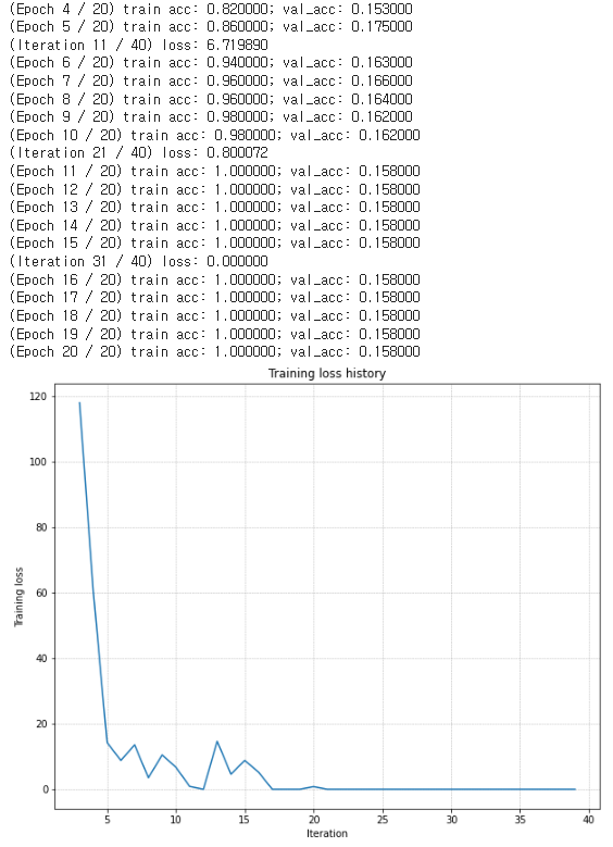
# TODO: Use a three-layer Net to overfit 50 training examples by
# tweaking just the learning rate and initialization scale.

num_train = 50
small_data = {
  "X_train": data["X_train"][:num_train],
  "y_train": data["y_train"][:num_train],
  "X_val": data["X_val"],
  "y_val": data["y_val"],
}

weight_scale = 1e-1   # Experiment with this!
learning_rate = 1e-3  # Experiment with this!
model = FullyConnectedNet(
    [100, 100],
    weight_scale=weight_scale,
    dtype=np.float64
)
solver = Solver(
    model,
    small_data,
    print_every=10,
    num_epochs=20,
    batch_size=25,
    update_rule="sgd",
    optim_config={"learning_rate": learning_rate},
)
solver.train()

plt.plot(solver.loss_history)
plt.title("Training loss history")
plt.xlabel("Iteration")
plt.ylabel("Training loss")
plt.grid(linestyle='--', linewidth=0.5)
plt.show()
모델을 잘 만들었는지 확인하기 위해 3-layer network에서 적절하게 learning rate와 weight scale 를 조절하면, regularization이 없다는 가정 하에 적은 epoch (20) 으로도 train acc가 1에 가까운 완전히 overfit 된 model 을 만들 수 있다. 잘 나온 것을 볼 수 있다.
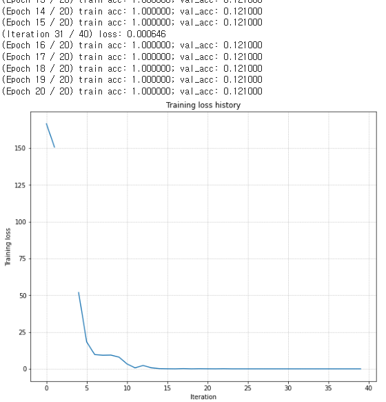
# TODO: Use a five-layer Net to overfit 50 training examples by
# tweaking just the learning rate and initialization scale.

num_train = 50
small_data = {
  'X_train': data['X_train'][:num_train],
  'y_train': data['y_train'][:num_train],
  'X_val': data['X_val'],
  'y_val': data['y_val'],
}

learning_rate = 2e-3  # Experiment with this!
weight_scale = 1e-1   # Experiment with this!
model = FullyConnectedNet(
    [100, 100, 100, 100],
    weight_scale=weight_scale,
    dtype=np.float64
)
solver = Solver(
    model,
    small_data,
    print_every=10,
    num_epochs=20,
    batch_size=25,
    update_rule='sgd',
    optim_config={'learning_rate': learning_rate},
)
solver.train()

plt.plot(solver.loss_history)
plt.title('Training loss history')
plt.xlabel('Iteration')
plt.ylabel('Training loss')
plt.grid(linestyle='--', linewidth=0.5)
plt.show()
다음은 5-layer network이다. 중간의 끊긴 부분은 아마 softmax함수에서 divide by zero가 일어 난 것 같다.
Inline Question 1:
Did you notice anything about the comparative difficulty of training the three-layer network vs. training the five-layer network? In particular, based on your experience, which network seemed more sensitive to the initialization scale? Why do you think that is the case?
Answer:
Three layer network is more difficult. Since we don't care about regularization and validation accuracy in this experiment, the more networks mean more weights, and more weights can classify train data better although they might not give a general prediction.
다음 문제는 3-layer net와 5-layer net 중 어떤 것이 더 overfit한 모델을 만들기가 어려웠는지 판단하는 문제이다. 내 생각은 3-layer net이 더 어렵다고 생각했다. 5-layer net이 weight가 더 많기 때문에, 그리고 여기서는 regularization을 고려하지 않기에 당연히 weight의 개수가 많은 5-layer net이 overfit한 model을 train하는데 더 쉬웠을 것이라고 생각했다.
def sgd_momentum(w, dw, config=None):
if config is None:
config = {}
config.setdefault("learning_rate", 1e-2)
config.setdefault("momentum", 0.9)
v = config.get("velocity", np.zeros_like(w))
next_w = None
# *****START OF YOUR CODE (DO NOT DELETE/MODIFY THIS LINE)*****
v = config['momentum'] * v - config['learning_rate'] * dw
next_w = w + v
# *****END OF YOUR CODE (DO NOT DELETE/MODIFY THIS LINE)*****
config["velocity"] = v
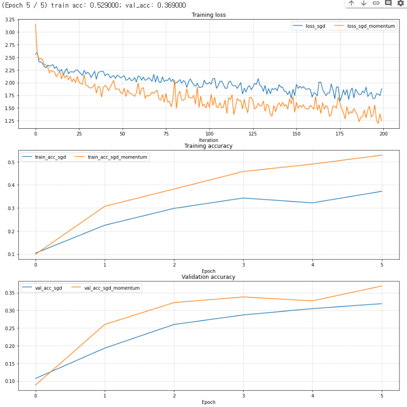
return next_w, config다음은 momentum sgd를 구현하는 문제이다. 공식을 따라하면 쉽게 구현할 수 있다. 밑의 사진은 gradient update에서 일반 SGD를 이용한 방법과 SGD momentum을 사용한 방법의 차이를 보여주는 그래프이다. SGD momentum을 이용한 방법이 loss를 줄이는데, training acc와 val acc를 올리는데 더 효과적인 것을 볼 수 있다.
다음은 gradient update의 또다른 방법인 adam() 함수를 구현하는 문제이다. 한번 update할때마다 t를 1씩 증가시켜 주고, 수식대로 m과 v를 계산하고 t에 따른 mt와 vt를 계산하고 업데이트 해 주면 된다.
def adam(w, dw, config=None):

    if config is None:
        config = {}
    config.setdefault("learning_rate", 1e-3)
    config.setdefault("beta1", 0.9)
    config.setdefault("beta2", 0.999)
    config.setdefault("epsilon", 1e-8)
    config.setdefault("m", np.zeros_like(w))
    config.setdefault("v", np.zeros_like(w))
    config.setdefault("t", 0)

    next_w = None
    # *****START OF YOUR CODE (DO NOT DELETE/MODIFY THIS LINE)*****

    config['t'] += 1
    config['m'] = config['beta1'] * config['m'] + (1- config['beta1']) * dw
    mt = config['m'] / (1-config['beta1']**config['t'])
    config['v'] = config['beta2'] * config['v'] + (1- config['beta2']) * dw**2
    vt = config['v'] / (1-config['beta2']**config['t'])
    next_w = w - ((config['learning_rate'] * mt) / (np.sqrt(vt) + config['epsilon']))

    # *****END OF YOUR CODE (DO NOT DELETE/MODIFY THIS LINE)*****

    return next_w, config
Inline Question 2:
AdaGrad, like Adam, is a per-parameter optimization method that uses the following update rule:
cache += dw**2
w += - learning_rate * dw / (np.sqrt(cache) + eps)
John notices that when he was training a network with AdaGrad that the updates became very small, and that his network was learning slowly. Using your knowledge of the AdaGrad update rule, why do you think the updates would become very small? Would Adam have the same issue?
Answer:
First few updates AdaGrad would work but as the iteration continues, you can see cache is keep increasing and stacking up dw**2s, which leads to denominator part of w update is keep increasing which will make small updates as it processes. Adam would not have this problem since it has mt = m / beta1^t and vt = m / beta2^t term. As iteration increase, denominators (beta1^t, beta2^t) decreases and scales up the m and v as iteration increases.
다음 문제는 주어진 코드의 Adagrad함수를 이용해서 업데이트 하면 AdaGrad에서 시간이 지날수록 update가 너무 작아지는데, 그 이유가 무엇인지, 그리고 Adam은 이 문제가 있는지 판단하는 것이다.
위의 Adagrad함수 식을 보면 cache가 계속해서 dw**2를 더해나가며 점점 커지는 것을 알 수 있다. 만약 train이 많이 진행되면, dw는 계속 쌓이므로 너무 커지게 되어, w += 에있는 분모의 sqrt(cache)가 너무 커지게 되어 update가 0에 수렴하게 되기 때문이다. Adam은 mt = m/beta^t, vt = m/beta2^t 수식이 있기 때문이 이런 문제가 없을 것이다. train을 진행할수록 (t 가 커질수록) mt, vt 의 분모가 점점 더 작게 조정되어 mt와 vt의 값이 커지기 때문에 m 과 v의 비율이 iteration이 지날수록 커지게 된다.
best_model = None

################################################################################
# TODO: Train the best FullyConnectedNet that you can on CIFAR-10. You might   #
# find batch/layer normalization and dropout useful. Store your best model in  #
# the best_model variable.                                                     #
################################################################################
# *****START OF YOUR CODE (DO NOT DELETE/MODIFY THIS LINE)*****
best_acc = -1

learning_rates = [1e-3, 1e-4]
weight_scale = [5e-2]
dropout_keep_ratio = [1, 0.5]
batch_size = [50,100]
normalize = [True, False]

for lr in learning_rates:
  for w in weight_scale:
    for bs in batch_size:
      for drop_p in dropout_keep_ratio:
        for bn in normalize:
          model = FullyConnectedNet(
                [100, 100, 100, 100, 100],
                weight_scale= w,
                dropout_keep_ratio = drop_p,
                normalization = bn)
          solver = Solver(
              model,
              data,
              num_epochs=10,
              batch_size=bs,
              update_rule='adam',
              optim_config={'learning_rate': lr},
              verbose=False)

          solver.train()

          acc = solver.check_accuracy(data['X_val'], data['y_val'], batch_size = 100)
          print('learning_rates:',lr,'weight_scale:',w, 'batch_size:', bs, 'dropout_ratio:', drop_p, 'batch_norm:', bn, 'acc:',acc)

          if acc > best_acc:
            best_acc = acc
            best_model = model

# *****END OF YOUR CODE (DO NOT DELETE/MODIFY THIS LINE)*****
################################################################################
#                              END OF YOUR CODE                                #
################################################################################
마지막으로 cross val을 이용해서 지금까지 배운 것을 사용해 최고의 FCnet을 만들어 보는 문제이다. 최소 50% validation accuracy가 나와야 된다고 한다.
나는 learning rate, weight scale, dropout, batch size, batch normalization을 변경해 가며 만들어 보았다. dropout = 1이면 dropout 사용을 안한다는 뜻이고, batch normalization = True, False에따라 batch norm을 사용하거나 사용하지 않는다.
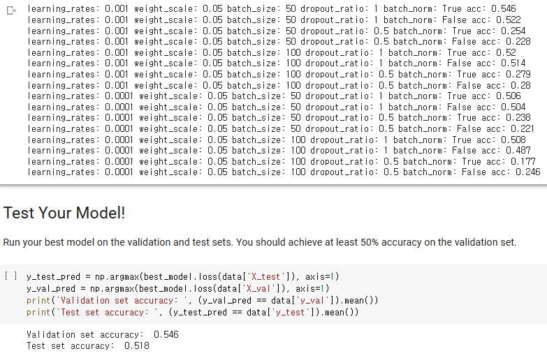
위와 같은 상태에서 validation accuracy 54.6 %, Test accuracy 51.8%가 되는 최고의 모델을 만들어 보았다.
'cs231n' 카테고리의 다른 글
| cs231n Assignment 2: Q3 (Dropout 구현) (0) | 2023.02.15 |
|---|---|
| cs231n Assignment 2: Q2 (Batch Normalization, Layer Normalization 구현) (0) | 2023.02.14 |
| cs231n Assignment 1: Q5 (HOG, HSV 추출 사용) (0) | 2023.02.06 |
| cs231n Assignment 1: Q4 (Two Layer Network 구현) (0) | 2023.02.01 |
| cs231n Assignment1: Q3 (Softmax layer, SGD 구현) (0) | 2023.02.01 |